
[Paper Review] Glow: Generative Flow with Invertible 1×1 Convolutions
논문 링크 : Glow
Glow: Generative Flow with Invertible 1×1 Convolutions 논문 리뷰입니다.
Introduction
기계학습 분야에서 해결되지 않은 두 가지 주요 문제가 있다.
- data efficiency : 인간처럼 적은 데이터로부터 학습할 수 있는 능력
- generalization : task나 context가 변경되었을 때의 강건함
AI system은 종종 학습데이터 분포와 다른 input이 주어지면 전혀 작동하지 않는 경우가 있는데, 생성 모델은 이러한 한계를 극복할 가능성을 가지고 있다.
- 현실적인 세계 모델을 학습하여 에이전트가 실제 세계와 상호작용하기 전에 계획을 세울수 있다.
- Input의 유의미한 특징을 거의 또는 전혀 인간의 supervision이나 labeling없이 학습할 수 있다.
생성 모델링 분야의 가능도 기반 방법은 세가지 범주로 나눌 수 있다.
- Autoregressive model : 단순하다는 장점이 있지만, 데이터의 차원 수에 비례하여 계산 시간이 증가한다.
- Variational autoencoders : 데이터의 log-likelihood 하한을 최적화한다.
- Flow-based generative model
Flow-based generative model의 장점
- Exact latent-variable inference and log-likelihood evaluation : VAE에서는 데이터 포인트에 해당하는 latent variable값을 근사적으로만 추론할 수 있다. 반면, reversible한 생성 모델에서는 근사없이 정확한 추론이 가능하며, 이를 통해 데이터의 log-likelihood를 정확한 값으로 최적화할 수 있다.
- 효율적인 추론과 생성 : Flow based 생성모델은 추론과 생성을 병렬화하기에 효율적이다.
- 유용한 latent space : 데이터 포인트 간의 interpolation 및 기존 데이터 포인트의 의미있는 수정과 같은 다양한 응용이 가능하다.
- 메모리 절약 : 네트워크의 깊이에 따라 선형이 아닌 일정한 양의 메모리만 필요하다.
Background: Flow-based Generative Models
고차원 random vector $\mathbf{x}$가 알려지지 않은 실제 분포 $\mathbf{x}\sim p^{\ast}(\mathbf{x})$를 따른다고 가정한다.
독립이고 동일한 분포($i.i.d$) 데이터셋 $\mathcal{D}$를 수집하고, parameter $\theta$를 가진 model $p_{\pmb{\theta}}(\mathbf{x})$를 선택한다.
- discrete data $\mathbf{x}$의 경우 아래와 같은 수식을 최소화 한다.
$$
\mathcal{L}(\mathcal{D})=\frac{1}{N}\sum^{N}_{i=1}-\log p_{\pmb\theta}(\mathbf{x}^{(i)})\tag{1}
$$
- continuous data $\mathbf{x}$의 경우 아래와 같은 수식을 최소화 한다.
$$
\mathcal{L}(\mathcal{D})\simeq \frac{1}{N}\sum^{N}_{i=1}-\log p_{\pmb\theta}(\tilde{\mathbf{x}}^{(i)}) + c \tag{2}
$$
- $\tilde{\mathbf{x}}^{(i)}=\mathbf{x}^{(i)}+u$ 이며, $u \sim \mathcal{U}(0,a)$ 이고, $c=-M\cdot \log a$이다.
- $a$는 데이터의 discretization level에 의해 결정된다.
- $a$가 작을수록 더 세밀하게 데이터를 나누고, 클수록 discretization 구간이 커진다.
- $M$은 $\mathbf{x}$의 차원수이다.
대부분의 flow-based 생성모델은 아래와 같은 수식으로 정의된다.
$$\begin{align}
\mathbf{z}\sim p_{\pmb{\theta}}(\mathbf{z}) \tag{3}\\
\mathbf{x}=\mathbf{g}_{\pmb{\theta}}(\mathbf{z})\tag{4}
\end{align}$$
- $\mathbf{z}$ : latent variable
- $p_{\pmb{\theta}}(\mathbf{z})$ : spherical multivariate Gaussian distribution과 같이 다루기 쉬운 density를 가진다.($p_{\pmb{\theta}}=\mathcal{N}(\mathbf{z};0,\mathbf{I})$)
- $\mathbf{g}_{\pmb{\theta}}$(..) : invertible (bijective)
- datapoint $\mathbf{x}$가 주어졌을 때, latent-variable 추론은 $\mathbf{z}=\mathbf{f}_{\pmb{\theta}}(\mathbf{x})=\mathbf{g}_{\pmb{\theta}}^{-1}(\mathbf{x})$로 수행된다.
$\mathbf{f}=\mathbf{f}_{1} \circ \mathbf{f}_{2}\circ \cdots \circ \mathbf{f}_{K}$ : sequence of transformations(likewise $\mathbf{g}$)
위와 같은 방식으로 $\mathbf{x}$와 $\mathbf{z}$사이의 관계는 아래와 같이 표현된다.
$$
\mathbf{x} \overset{\mathbf{f}_{1}} \longleftrightarrow \mathbf{h}_{1}\overset{\mathbf{f}_{2}} \longleftrightarrow \mathbf{h}_{2} \cdots \overset{\mathbf{f}_{K}} \longleftrightarrow \mathbf{z} \tag{5}
$$
위와 같은 invertible transformation을 normalizing flow라고 한다.
주어진 datapoint에 대해 모델의 pdf는 $\mathbf{h}_{0}=\mathbf{x}, \mathbf{h}_{K}=\mathbf{z}$라고 하면, 아래의 수식과 같이 쓸 수 있다.
$$\begin{align}
\log p_{\pmb{\theta}}(\mathbf{x}) &= \log p_{\pmb{\theta}}(\mathbf{z}) + \log \vert \det (d\mathbf{z} / d\mathbf{x}) \vert \tag{6} \\
&= \log p_{\pmb{\theta}}(\mathbf{z})+\sum^{K}_{i=1}\log \vert \det(d\mathbf{h}_{i} / d\mathbf{h}_{i-1})\vert\tag{7}
\end{align}$$
수식을 간단하게 분석하면, 아래와 같다.
$$\begin{align}
p_{\pmb{\theta}}(\mathbf{x})&=p_{\pmb{\theta}}(\mathbf{h}_{1})\cdot \vert \det(d\mathbf{h}_{1}/d\mathbf{x})\vert\\
p_{\pmb{\theta}}(\mathbf{h}_{1})&= p_{\pmb{\theta}}(\mathbf{h}_{2})\cdot \vert \det(d\mathbf{h}_{2}/d\mathbf{h}_{1})\vert\\
\log p_{\pmb{\theta}}(\mathbf{x})&= \log p_{\pmb{\theta}}(\mathbf{h}_{1}) + \log \vert \det(d\mathbf{h}_{1}/d\mathbf{x})\vert\\
&= \log p_{\pmb{\theta}}(\mathbf{h}_{2}) + \log \vert \det(d\mathbf{h}_1/d\mathbf{x})\vert+
\log \vert \det(d\mathbf{h}_{2}/d\mathbf{h}_{1})\vert
\end{align}$$
$\log \vert \det (d\mathbf{h}_{i}/d\mathbf{h}_{i-1})\vert$은 삼각행렬을 사용하는 특정 변환을 통해 간단하게 계산된다.
$$
\log \vert \det (d\mathbf{h}_{i}/d\mathbf{h}_{i-1})\vert=
\text{sum}(\log \vert \text{diag}(d\mathbf{h}_{i}/d\mathbf{h}_{i-1})\vert)\tag{8}
$$
Proposed Generative Flow
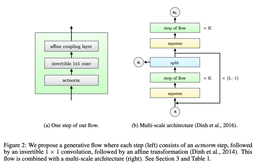
제안한 flow는 multi-scale architecture에 결합된 flow 단계들로 구성된다.
- actnorm
- invertible 1x1 conv
- affine coupling layer
Multi-scale architecture는 flow depth $K$와 level의 수$L$ 을 가지고 있다.
Actnorm: scale and bias layer with data dependent initialization
이전의 연구에서는 batch normalization을 사용하였지만, activation에 추가된 noise의 분산은 PU 당 minibatch 크기에 반비례하므로, 크기가 작을때 성능이 저하되는 것으로 알려져 있다. large image에 대해 메모리 제약으로 PU당 minibatch가 1로 설정된다. 이에 actnorm(activation normalization)을 제안한다.
각 channel별로 scale과 bias를 사용하여 activation에 대해 affine transformation을 수행한다. 이 parameter들은 초기 minibatch가 주어졌을 때, 각 channel별로 평균이 0이고, 분산이 1이 되도록 초기화된다. 초기화 후에는 scale과 bias는 data와 독립적으로 학습가능한 parameter로 처리된다.
Invertible 1x1 convolution
이전 연구에서는 고정된 permutation을 제안했다. 이 논문에서는 고정된 permutation이 아닌 학습가능한 invertible 1x1 convolution을 제안한다.
weight matrix는 random rotation matrix로 초기화 되며 1x1 convolution은 input channel과 output channel의 수가 같을 때 permutation operation의 일반화 형태이다.
$h \times w \times c$ tensor $\mathbf{h}$와 $c \times c$ weight matrix $\mathbf{W}$의 행렬식은 아래와 같이 간단하게 계산할 수 있다.
$$
\log \left \vert \det \left(\frac{d \text{conv2D}(\mathbf{h};\mathbf{W})}{d\mathbf{h}}\right)\right \vert=h\cdot w\cdot \log \vert \det(\mathbf{W}) \vert \tag{9}
$$
LU Decomposition
$\det(\mathbf{W})$의 계산비용을 LU분해를 통해 $\mathbf{W}$를 파라미터화 하여 $\mathcal{O}(c^{3})$ 에서 $\mathcal{O}(c)$로 줄일 수 있다.
$$
\mathbf{W}=\mathbf{P}\mathbf{L}(\mathbf{U}+\text{diag}(\mathbf{s}))\tag{10}
$$
- $\mathbf{P}$ : permutation matrix(행의 순서를 바꾸는 순열행렬)
- $\mathbf{L}$ : 대각원소가 1인 하삼각행렬
- $\mathbf{U}$ : 대각원소가 0인 상삼각행렬
- $\mathbf{s}$ : $\mathbf{U}$의 대각원소값을 가지는 vector
$$
\log \vert \det(\mathbf{W})\vert=\text{sum}(\log \vert \mathbf{s}\vert) \tag{11}
$$
이 parameterization에서 random rotation matrix $\mathbf{W}$를 샘플링하고, 고정된 $\mathbf{P}$값을 계산한 후, 초기 $\mathbf{L},\mathbf{U},\mathbf{s}$값을 최적화 하는 방식으로 설정한다.
큰 $c$에 대해서는 비용차이가 나지만, 논문에서의 실험은 계산 비용이 크게 차이 나지 않았다.
Affine Coupling Layers
forward function, reverse function, log-determinant가 계산적으로 효율적인 reversible transformation은 Affine Coupling Layer이다.
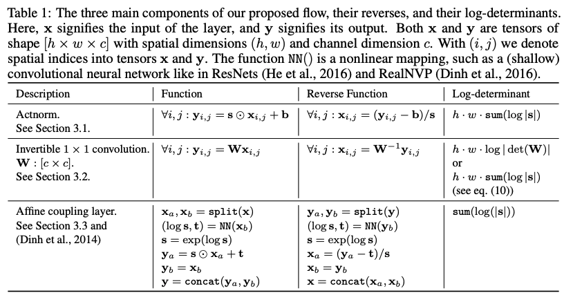
additive coupling layer는 특수한 경우로 $\mathbf{s}=1$일 때 log-determinant가 0이되는 경우이다.
Zero initialization
각 신경망의 마지막 convolution을 0으로 초기화하여, 각 Affine coupling layer가 초기에는 identity function으로 수행한다. (이것이 매우 깊은 network를 학습할 때 도움이 된다는 것을 발견했다.)
Split and concatenation
Split 함수는 input tensor $\mathbf{h}$를 channel 차원에서 두 개로 나눈다. concat 함수는 나눠진 tensor를 하나의 tensor로 다시 결합한다.
이 연구에서는 channel 차원에서만 분할을 수행하여 전체 architecture를 단순화 했다.
Permutation
위의 각 step of flow는 변수의 permutation을 선행해야한다. 이는 flow가 충분한 step후에 각 차원이 다른 모든 차원에 영향을 줄 수 있도록 하기 위함이다.
이전 연구에서 수행된 permutation 방식은 channel(feature)의 순서를 단순히 뒤집은 것과 동일하다. 대안으로는 fixed random permutation이 있다. 본 논문에서는 Invertible 1 x 1 convolution은 이러한 permutation의 일반화이다.
Quantitative Experiments
실험에서 Glow와 RealNVP가 어떻게 비교되는지 알아보았다.
그런다음, model을 표준 dataset에 적용하고, 이전의 생성 모델들과 log-likelihood를 비교하였다.
각 $\text{NN}$()에 3개의 convolution layer를 사용하며, 2개의 hidden layer는 ReLU activation function과 512 channel을 가진다.
Gains using invertible 1 x 1 Convolution
channel 변수들의 permutation에 대해 세가지 변형을 고려하였다.
- RealNVP에서의 reversing operation
- fixed random permutation
- invertible 1 x 1 convolution
CIFAR-10에서 평균 negative log-likelihood를 비교하였다.
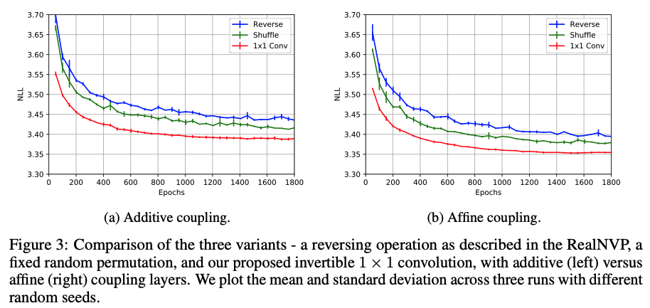
additive coupling layer만을 사용한 모델과, affine coupling을 사용한 모델을 위 그림과 같이 비교하였다. 그림에서 볼 수 있듯이 invertible 1x1 convolution이 더 낮은 negative log-likelihood를 달성하며 더 빠르게 수렴했다.
Qualitative Experiments
고해상도 dataset에서 모델의 qualitative 측면의 연구이다.
모델이 고해상도로 확장 가능한지, 현실적인 샘플을 생성할 수 있는지, 의미있는 잠재 공간을 생성할 수 있는지에 대한 실험이다.
특히, Semantic Manipulation에서 smiling, Blond hair 등 속성의 유무에 따른 latent vector를 이용하여 다양한 속성을 매우 쉽게 적용하였다.
$\mathbf{v}_{att}= \mathbf{z}_{pos}-\mathbf{z}_{neg}$ 라고 한다면, $\mathbf{z}_{original}+\alpha \mathbf{v}_{att}$를 추가하여 해당 속성의 변화를 얻을 수 있다.
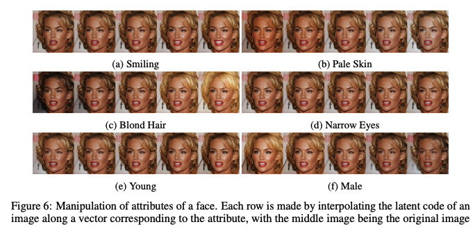
가운데 image가 original image이다.
Conclusion
- 새로운 유형의 generative flow를 제안하여 log-likelihood 측면에서 개선된 성능을 입증한다.
- 또한, 고해상도의 이미지를 학습했을 때, 현실적인 이미지를 합성할 수 있다.